CNN Locality and Inductive Bias

This post was migrated from Tistory. You can find the original here.

CNN Locality

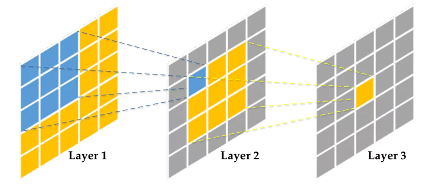
In a CNN, the feature at a given pixel location is computed from a local patch of the input image,

and the extent of the input region that influences that output is called the receptive field.

Early layers only look at small patches, but as layers get deeper, the receptive field keeps expanding,

so the feature at each location ends up integrating information from an increasingly wide region of the input.

Receptive Field Expansion and Global Relationships

As shown above, a single pixel in layer3 corresponds to the entire layer1.

It’s true that the receptive field grows larger as layers get deeper, but

let’s take a 1D example with [A, B, C, D, E].

CNN

D, E → C → B → A

Information from far away propagates to A through its neighbors, step by step.

CNNs only convey global relationships indirectly.

y(i,j) = Σ_k Σ_l W(k,l) · x(i+k, j+l)
The output at (i,j) only uses the neighborhood around (i+k, j+l)
The range of k, l = kernel size

(Comparison) Self-Attention

{B, C, D, E} (direct weighted sum) → A

Every position is directly connected to every other position, integrating information via a weighted sum.

y_i = Σ_j α(i,j) · x_j
Position i directly references every position j
The range of j = the entire input, every position in the input sequence

CNN Locality Inductive Bias

Why does the locality bias make sense? → Because of the statistical properties of natural images.

• Low-level visual patterns like edges, corners, and textures tend to exist locally.
• Nearby pixels have a strong statistical correlation with each other.

How does a CNN inject this inductive bias? → By baking the assumption into its architecture.

• The assumption “nearby pixels carry more relevant information for each other” is enforced structurally.
• Convolutional kernels are applied only to local regions, and the same kernel is shared across the entire spatial extent (stationarity).

What are the benefits of designing an inductive bias this way?

The locality inductive bias greatly narrows the hypothesis space the model has to search, enabling efficient learning even with limited data.

Also, since the convolution operation has linear computational complexity with respect to spatial size, the compute cost scales predictably even for high-resolution images.

Structural Limitations of the CNN Locality Inductive Bias

Let’s use both eyes as an example.

CNN

Features for the left eye and the right eye are each extracted locally,

then gradually merged in deeper layers, becoming implicitly combined.

The relationship between the two eyes propagates indirectly through many layers,

and the fact that “there are two eyes” is inferred as a byproduct of combining patterns.

(Comparison) Self-Attention

The left eye and the right eye form a direct attention edge,

so the relationship between the two locations is explicitly modeled as a graph structure.

Summary

So for problems where global relationships matter, such as:

• Symmetry between lesions in the left and right lung
• Long-range dependencies in a sentence
• Reasoning about relationships between distant objects

CNNs need deeper networks, gradient paths get longer, and data requirements increase as well.

Also, because the relationship is represented implicitly,

it’s hard to verify whether it was actually learned well, and without a clear evaluation criterion for the relationship,

it becomes difficult to form solid hypotheses for experiments around data composition, sampling ratios, model architecture, and so on.

+ GAP (Global Average Pooling)

Inductive bias shows up not just in the backbone representation but also at the feature aggregation stage.
Global Average Pooling (GAP) is a feature pooling operation mainly used in classification models.

It averages the spatial dimensions (H×W) of each channel (feature map) down to a single scalar value per channel.

Each channel represents the activation tendency for a specific visual pattern (e.g., an edge, a texture, part of an object’s structure),

and GAP globally summarizes how strongly that pattern is present across the whole image.

Positional information is discarded, and only the strength of the pattern’s presence is preserved.

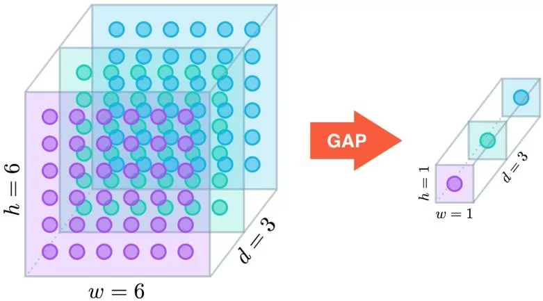
Feature Map: (C × H × W) → Vector: (C)

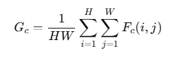
This isn’t an operation that removes channels or merges information across channels —
it summarizes the spatial dimensions (H×W) of each channel individually, and the positional information for (i, j) disappears.

Why is it mainly used for classification problems?

In classification, what matters is presence rather than location — e.g., “Is there a cat in this image?”

The Flatten + Fully Connected (FC) combination flattens the (H×W×C) feature map as-is,
producing a huge number of FC parameters, which increases model size and the risk of overfitting.

GAP, on the other hand, reduces the (H×W×C) feature map down to a (C)-dimensional vector,
cutting down the parameter count, memory usage, and overfitting risk all at once.

It also reduces dependence on any specific location by averaging out spatial information,
strengthening translation invariance and providing an inductive bias that benefits classification generalization.